 |
SyTen
|


|
|
SyTen
|
|
The toolkit supports four different criteria based on which it discards singular values. Any of these criteria is sufficient to discard a particular singular value. Two are only sensible relative to the norm of the input tensor, which is why it is useful to call Truncation::scale() prior to a SVD, passing in the norm of the tensor.
The four criteria are:
truncMaxBlocksize or b in DMRG stage stanzas, somtimes -b option: If the maximal size of a dense block exceeds this size, the smallest singular values are discarded.truncMaxStates or m in DMRG stage stanzas, usually -m option: If the sum of the sizes of all dense blocks exceeds this size, the smallest singular values are discarded.truncThreshold or t in DMRG stage stanzas, usually -t option: If a singular value is smaller than this, it will be discarded.truncWeight or w in DMRG stage stanzas, usually -w option: The smallest singular values are discarded until the sum of their squares reaches just below this value. Note that this is usually a very small number. If you truncate a normalised MPS with specified weight \( \omega \), you will incur an error \( \sqrt{\left|\left| \left|\psi\right\rangle -
\left|\psi^\prime\right\rangle \right|\right|} \) of approximately \( \sqrt{2 L \omega} \).Also note that the error typically reported is calculated as \(
\left( \sum_{i=1}^L \right) \sqrt{2 - 2 \sqrt{1 - \omega/N^2}} \) where \(N\) is the norm of the state and we either report a single truncation (without the sum) or the maximal accumulation of all truncations (with the sum). This is of roughly the same order as \(
\sqrt{2 L \omega} \), but in the case of multiple truncations, both expressions are upper bounds, not the exact error. You can get the exact error from syten-overlap --norm --subtract original.mps truncated.mps which calculates \( 1 - \left\langle \psi^\prime
\middle| \psi \right\rangle / \left(\left|\left|
\left|\psi\right\rangle \right| \right| \cdot \left|\left|
\left|\psi^\prime\right\rangle \right| \right|\right) \). Taking the square root of this value will give you the approximate error.
Many tools require a tensor product operator (at the moment either MPO or BTTO) as an input. Tensor product operators are stored in lattice files and are accessed using the generic <lattice file>:<operator expression> syntax. <lattice file> here is the usual name of the file, <operator expression> can be the name of a specific global operator or a more complicated expression. This expression is parsed using reverse prefix notation. That is, assuming two operands a and b and a binary operation f, the result f(a, b) is expressed in this syntax as b a f. RPN has the advantage that no parantheses are necessary to uniquely specify operation ordering and that writing a parser for it is extremely simple. For example, the expression I 3 * takes the identity operator from the lattice and multiplies it by three. The expression I 3 * H + does the same as above and then adds the result to the operator defined on the lattice as H.
The operand types of the operator parser are:
H or q3,03 or (0,-2.123e-4)By default, each element of the operator expression is interpreted as a number unless that conversion fails. If this conversion fails, the element is stored as a string. Strings can implicitly be converted to numbers, sectors and TPOs. If after evaluation of all operations the final operand is not a TPO, it will implicitly be converted into a TPO.
For matrix product operators, the following functions/operators are available:
<x> ? or <x> _operator: explicitly interprets the string <x> as a global TPO. Example: H ?, N ?, both equivalent to just H and N.<x> <y> @ or <x> <y> _at_site: if <y> can be parsed as a number, constructs the single-site operator <x>_<y>, otherwise constructs the single-site operator <y>_<x>. Example: sz 0 @, 17 s @, n 2 _at_site.<x> # or <x> _sector: Converts <x> starting at its second position into a quantum number sector description with respect to the current lattice. Example: q0,3 or a15. Note that the first position is ignored but necessary to avoid interpreting e.g. 15 as a number (which cannot be converted into a sector any more).<x> … or <x> _distribute. Builds the MPO \( x \mathbb{1} \), i.e. the identity times <x>, with the absolute value of the factor distributed evenly over all tensors. The phase is stored in the first tensor. Example: 15 _distribute.<x> : or <x> _truncate. Explicitly truncates the MPO <x>, even if the parsing component was invoked with truncation disabled. Useful to (pre-)truncate the arguments for syten-truncate or syten-print, which normally don't truncate in the parser. Example sz 0 @ sz 1 @ + _truncate.<a> <b> + adds two numbers or two operators together.<a> <b> * or <a> <b> _mult. If <a> and <b> are both numbers, calculates the product of the two numbers. If one is an operator and the other a number, scales the operator by the number. If both are operators, calculates \( a b \) (or, in SyTen C++, b * a). That is, <b> is applied first and <a> is applied second. Example: 2 3 * is 6, 4 I * is the identity scaled by four, A B * is \( A B (|\psi\rangle)\), chu 0 @ cu 0 @ * is nu 0 @.<a> <b> · or <a> <b> _dot calculates the dot product of two operators <a> and <b> as dot(b, a), which applies b first and dual-space-conjugated a second. Example: c 0 @ c 1 @ _dot is \( c_0^\dagger \cdot c_1 \), if the dual-space conjugate of cu is chu, cu 1 @ cu 0 @ _dot is the same as chu 1 @ cu 0 @ *. If <b> is already a sector, the function forwards to _dotq, see below.<a> <b> <q> _dotq calculates the dot product of two operators <a> and <b> projected into the sector <q> as dot(b, a,
q). Example: c 0 @ c 0 @ q0,1 _dotq is proportional to s 0 @ in a Fermi-Hubbard system and hence c 0 @ c 0 @ q0,1 _dotq c 0 @ c 0 @ q0,1 _dotq _dot 0.75 * is the same as s 0 @ s 0 @ _dot or \(
(\hat s_0)^2 \). The first position of <q> is ignored but potentially necessary to avoid interpretation as a number. The string following the first position is interpreted in exactly the same way as in e.g. syten-random -s or syten-apply-op -s.<a> ^m2 or <a> _msquare is the same as <a> <a> *, i.e. calculates the square of a number or an operator. Example: H 1.2345 -1 * _distribute _msquare calculates \( \left( \hat H -
1.2345 \right)^2 \).<a> ^d2 or <a> _dsquare calculates either dot(a, a) (for operators) or a * conj(a) (for numbers).For binary tree tensor operators, the following operations are defined:
<x> ? or <x> _operator: explicitly interprets the string <x> as a global TPO. Example: H ?, N ?, both equivalent to just H and N.<x> <y> @ or <x> <y> _at_site: if <y> can be parsed as a number, constructs the single-site operator <x>_<y>, otherwise constructs the single-site operator <y>_<x>. Example: sz c2:3 @, c17:1 s @, n c2:1 _at_site. For details of the accepted coordinates, see operator[].<x> # or <x> _sector: Converts <x> starting at its second position into a quantum number sector description with respect to the current lattice. Example: q0,3 or a15. Note that the first position is ignored but necessary to avoid interpreting e.g. 15 as a number (which cannot be converted into a sector any more).<a> <b> * or <a> <b> _mult. If <a> and <b> are both numbers, calculates the product of the two numbers. If one is an operator and the other a number, scales the operator by the number. If both are operators, calculates \( a b \) (or, in SyTen C++, b * a). That is, <b> is applied first and <a> is applied second. Example: 2 3 * is 6, 4 I * is the identity scaled by four, A B * is \( A B (|\psi\rangle)\), chu c0:0 @ cu c0:0 @ * is nu c0:0 @.<a> <b> · or <a> <b> _dot calculates the dot product of two operators <a> and <b> as dot(b, a), which applies b first and dual-space-conjugated a second. Example: c c0:0 @ c c0:1 @ _dot is \( c_0^\dagger \cdot c_1 \), if the dual-space conjugate of cu is chu, cu c0:1 @ cu c0:2 @ _dot is the same as chu c0:1 @ cu c0:2 @ *. If <b> is already a sector, the function forwards to _dotq, see below.<a> <b> <q> _dotq calculates the dot product of two operators <a> and <b> projected into the sector <q> as dot(b, a, q).<a> <b> + adds two numbers or two operators together.Hkin and Hint as global operators in the lattice. The full Hamiltonian can then be constructed on the command line as $ syten-dmrg -l fh:'Hkin Hint 4 *' …for \( \hat H_{\mathrm{kin}} + 4 \hat H_{\mathrm{int}} \). The parameter can then be changed as desired from the command line without regenerating the lattice.
sz 2 @ for \( \hat s^z_2
\) on a \(\mathrm{U}(1)_{S^z}\)-symmetric spin lattice._dot may be used to dual-space conjugate an operator: A I _dot multiplies operators A and the identity I (defined on every lattice), but dual-space conjugates A in the process. The result is the proper \( A^\dagger \)._dot and _dotq may also be used to project an operator onto a specific quantum number sector, e.g. I A q4 _dot effectively projects A onto the 4 sector.The decision whether to use real scalars in tensors (double) or complex scalars (std::complex<double>) is currently a compile-time decision, i.e. there is no run-time introspection. This implies that once you decided to use real-valued scalars, you cannot do certain things to your wave function, e.g. apply an operator which requires complex numbers or do real-time evolution.
In comparison, if you are using only complex-valued scalars, all these things are possible even if you did not initially think of them. Hence, by default, the toolkit uses complex scalars. If you are sure that you only want to use real-valued scalars in your tensors, set -DSYTEN_COMPLEX_SCALAR=0 (c.f. SYTEN_COMPLEX_SCALAR).
Short answer: Use syten-tdvp or syten-krylov (for gapped systems or if your error requirements are very stringent). If you only wish to do imaginary-time evolution, consider SYTEN_COMPLEX_SCALAR.
Long answer: There are currently five time evolution implementations in the toolkit:
syten-tebd: Implements the classical TEBD algorithm and a real-space parallelised variant thereof of orders 1, 2 and 4, but requires the time-evolution operator (usually the Hamiltonian) to be split by hand into an ‘even’ and an ‘odd’ part, with those parts saved as individual MPOs in the toolkit. Furthermore, it currently only works on spin chains, as it requires all local operators occurring in the Hamiltonian ( \( \hat S^z, \hat S^+, \hat S^-\) etc.) to have zero overlap with the identity, i.e. \(
\mathrm{tr}\left( \hat O \hat I \right) = 0 \). Consider this to be currently in the testing phase, though it should work (at least the unparallelised method) reliably if your system permits it.syten-tebd-swappable: Also implements the standard TEBD algorithm (1st and 2nd order) but handles long-range interactions and arbitrary bosonic systems (Fermions may also work, I don't know). Requires an explicit list of summands of the Hamiltonian to be written to a text file first, which is then parsed and each summand exponentiated individually. See commit 00b6ea17 for details regarding the terms file. Unfortunately due to the inherent TEBD error of O(t^2) at best, it requires smaller time-steps than those which would be possible using the Krylov method and hence is usually slower.syten-tdvp: Based on the TDVP principle applied to MPS as described by Jutho Haegemann et.al. Both the one-site and two-site variants are implemented. The one-site variant is very fast, but incurs a fairly large error, as it does not increase the bond dimension. The two-site variant is slower, but supposedly exact if there are only nearest-neighbour interactions. However, we currently do not quantify the projection error properly.syten-taylor: Based on a simple Taylor series expansion of \(
\hat U = \mathrm{exp}\left\{ -i \hat H t \right\} \) and then repeated application of the constructed \( \hat U \). Extremely fast if you need many very short time steps, but the error is not well-controlled – what may seem like a decent time evolution may veer of uncontrollably within just a few time steps. Worse, changing the timestep just slightly may completely alleviate the problem. However, if the time step is very small and you need very many steps, the method has the advantage of only building \( \hat U
\) once in the beginning.syten-krylov: Based on the MPS-supported Krylov subspace method. At each step, the Krylov subspace is built up and the Hamiltonian exactly diagonalised within this subspace. The method is well-controlled and you can in principle push every error to zero. In principle, the method allows arbitrarily large time steps, but may require very many Krylov vectors (iterations) to achieve this result. Various options for the internal eigensolver are available, check the output of syten-krylov --help, but the defaults should work reliably, though not necessarily as fast as possible. If your iteration exits with "maxIter" (last column of output), decrease the size of the time step or increase the maximal number of Krylov vectors to achieve a converged result. If your initial state is reasonably complex, you may want to try the 'W' or 'V' orthonormalisation submodes instead of the default 'A' mode. The method works best in gapped systems with little entanglement.DMRG and MPS in general are methods which require low entanglement in the system to efficiently represent states. This means that while e.g. for ED solvers matrix dimensions \( 400 \times 400\) may be no problem, DMRG visibly starts to struggle if the dimension of the dense subblocks of its tensors exceeds \( \approx 500\). There are two ways to reduce this size (given as the last-but-one column in DMRG output):
Further, depending on your system, you may benefit from settings which are not the default settings:
expandBlocksize value (shortcut: eb) to something smaller like 10 or 20. Conversely, if you observe the number of blocks or the ratio between SU(2) and U(1) states getting very large, consider setting it to something larger. This value sets the maximal size by which each symmetry sector is enlarged during each iteration. A smaller value grows the sectors more slowly but also tends to prefer (e.g.) larger spin sectors, while a larger value causes the bond dimension to grow very quickly and favours the most important sectors. Note that the value here is always limited by the maximal number of states selected and the maximal blocksize allowed during truncation to avoid pointless expansion. If your state is sufficiently large, you may also set the expandRatio (shortcut: er) to something smaller from its default value of 0.5. This further limits the size of the expansion blocks, but in a more uniform way as it selects a fixed ratio of each block. However, for small states, it also over-estimates smaller blocks (due to a clipping of a minimal expansion of 1 required to get out of a product state).mode K submode A) should be the default, but both the Davidson method (mode D) or the matrix-based reorthogonalisation of the old 'classic' Lanczos implementation (mode C submode M) may be faster. To set these, look at the eigensolver stanza in the stages configuration. Note however that in particular the matrix-based reorthogonalisation may be unstable. On some systems, the Davidson method converges much better and to the actual ground state, while the Lanczos method will get stuck in a highly-excited state.(m 200 v 2DMRG) for m=200 states and a 2DMRG solver.syten-dmrg --help for details.Using both profile-guided optimisation and link-time optimisation helps a little bit with GCC (approx. 5%). To enable this, first add the line
CPPFLAGS_EXTRA+=-fprofile-generate
to your make.inc file, recompile and run a "typical" DMRG calculation. This will be slower than usual, so maybe restrict the number of sweeps. When completing, a number of *.gcda files will be created next to the compiled object files. Once this has been done, replace the line above by
CPPFLAGS_EXTRA+=-fprofile-use -flto -fno-fat-lto-objects
and recompile again. This will use the run-time timing information to slightly optimise your code. Especially in larger calculations where most time is spent inside BLAS/LAPACKE functions, the impact will be minimal, though.
First, add -ggdb3 to the CPPFLAGS_EXTRA variable in your make.inc file and ensure that you also added -DDEBUG and -Og. Before running your program, set the environment variable SYTEN_USE_EXTERN_DEBUG to disable the built-in signal and termination handler (which normally prints backtraces) and not unwind the stack and exit once an error occurs.
Then run gdb as normal, e.g. gdb --args syten-dmrg -l lat:H.... To print C++ objects, you can define a cpp_print function e.g. as follows:
> define cpp_print
> call (void)operator<<(std::cerr, $arg0)
> printf "\n"
> end
which you can then use with any local variable whose operator<< is compiled in (at least if they are simple, I didn't manage to print tensors this way). To get a list of local variables, use info locals. Make sure to also read any of the GDB tutorials/documentation writeups available online.
In principle, a physical symmetry can be used in a MPS if it is possible to assign each state of the MPS a single quantum number. For example, particle number conservation may be used if it is possible to assign each local physical state a single particle number. Momentum conservation on a ring can only be used after a Fourier transformation into momentum space, since otherwise the real-space states do not have definite momentum quantum numbers.
Currently implemented are \( \mathrm{SU}(3) \), \( \mathrm{SU}(2) \), \( \mathrm{U}(1) \) and \( \mathbb{Z}_k \) symmetry groups (note that the latter in particular also includes parity). Any local physical symmetry associated to any of these groups can be used without additional effort. Other groups ( \( \mathrm{SO}(3), \mathrm{Sp}(6)\) etc.) should be implementable without too much effort.
There are three alternative approaches to storing and writing data to and from disks:
There are only pairwise tensor contractions, i.e. expressions C = A·B. The basic interface for these contractions is the prod<C>(a<F>, b<S>, c_a, c_b) function which takes two tensors of ranks F and S and arrays of integers of the same size as well as the number of contracted tensor legs as an explicit template parameter C. Legs i of a and j of b are then contracted if c_a[i] == c_b[j] and c_a[i] > 0. A leg i of a becomes the k-th leg of the resulting tensor if c_a[i] == -k, similarly a leg j of b becomes the k-th leg of the resulting tensor if c_b[j] == -k. For example, to implement \( C_{ik} = \sum_{j} A_{ij} B_{jk} \), say C = prod<1>(A, B, {-1, 1}, {1, -2}). Each tensor leg has an associated direction, one can only contract an outgoing with an incoming index and vice versa, not two outgoing indices nor two incoming indices. prod<>() takes an additional boolean value which, if true, complex-conjugates the second argument and considers the directions of the legs of the second tensor to be inverted. By default, this flag is false.
Complete products (resulting in a scalar value) are available in two variants: prod<C>(a<C>, b<C>) calculates \( A \cdot B \) assuming that the order of legs matches between a and b and complex-conjugates b by default. Alternatively, it is also possible to specify all legs as contracted in the arrays c_a and c_b above which allows for products where the order of indices does not match between a and b. In this second form, b is not complex-conjugated by default. \( \mathrm{Tr}(A B^\dagger) \) can then be written as either prod<2>(a, b, {1, 2}, {1, 2}, true) or prod<2>(a, b[, true]).
There are two convenience wrappers around this basic prod<>() function:
The first, instead of integer arrays c_a and c_b takes two maps from indices to integers, this allows for an arbitrary order of these indices and hence does not require knowledge of the tensor order (only a global variable or function evaluating to the correct leg value). The matrix-matrix multiplication above could then be written as prod<1>(a, b, {{1, -1}, {2, 1}}, {{2, -2}, {1, 1}}).
The second takes either three strings or one string describing the tensor contraction using Einsteins summation convention. The variant with just one string immediately splits the string into three substrings at | characters and then behaves like the former. The index names can have arbitrary length and contain all characters but , which is used to separate the different indices. The matrix-matrix product above could be written as prod<1>(a, b, "i,j|j,k|i,k") or prod<1>(a, b, "i,j", "j,k", "i,k") or prod<1>(a, b, "first,summed|summed,second|first,second"). When using this form to initialise a complete product, the result index string has to be empty, i.e. prod<2>(a, b, "a,b|a,b|", true) or prod<2>(a, b, "first,second", "first,second", "", true).
fs and io2 are exactly identical in the following:The order of contraction of indices is rather important in tensor networks. For example, when calculating the norm of a matrix product state, it is paramount to contract from left to right all site tensors with their complex conjugate and the relevant transfer matrix, rather than first contracting all sites tensors, then all complex conjugates of all site tensors and then the two now-massive tensors representing the state together. While the former runs in polynomial time (linear in the length of the MPS, qubic in its bond dimension, linear in its physical dimension), the latter runs in exponential time in the length of the MPS! Similar differences can often occur in smaller networks when it is possible to contract multiple tensors in different ways.
While for small networks, the optimal ordering is fairly easy to figure out by hand (simply check the cost of all possible orderings), for larger networks, this gets complicated quickly.
In the source of arXiv:1304.6112v6, you will find a netcon.m file. Open this file in Matlab ($ module load matlab; matlab, then click it…). You then get a function netcon which is explained in more detail also in that paper. Essentially, a call:
netcon({[1,2,3],[4,5,6],[1,5,7,8,-1],[2,4,7,-2],[3,6,8,-3]},
       2,1,1,0,[1 w; 2 m; 3 m; 4 m; 5 w; 6 m; 7 d; 8 d; -1 v; -2 n; -3 n])
specifies that you have five tensors in your network (the five groups enclosed in [] in the first argument). The first tensor has indices labelled 1, 2 and 3; the third tensor has indices labelled 1, 5, 7, 8 and -1. Indices labelled with positive integers are contracted (e.g. the first indices of tensors one and three are to be contracted), while negative integers denote resulting tensor legs (the last leg of the third tensor is the first leg of the resulting tensor). The options in between shouldn't have to be changed, the last option denotes the dimensions of each index (labelled by positive and negative integers), e.g. index -1 has dimension v whereas index 2 has dimension m. You can change and assign to these variables as you please; for example
w = 3; v = 6; m = 100; n = 200; d = 2;
works for assignment. Once you call netcon(), it should give you a result relatively quickly, naming the indices in the order in which you should contract them, i.e.
Best sequence:  6 3 1 5 8 2 4 7
 Cost:           10032000000
means to first contract over index 6 (tensors 2 and 5), then index 3 (tensors 1 and (25)), followed by indices 1, 5 and 8 (tensor 3 and (125)) and finally indices 2, 4 and 7 (tensor 4 and (3125)).
There doesn’t seem to be an analytic option to this, but using hugely different orders of magnitude for different indices works equally well as specifying \( m \gg d \) in some imaginary language.
The above section deals with the order in which multiple tensors should be contracted together. This section deals with the ordering of legs within a tensor for optimal contraction. It is based on the fact that each dense tensor block is stored internally as an array of scalar numbers. When two dense tensor blocks are contracted together, the numbers in the two arrays have to be reshuffled such that the tensor contraction can be expressed as a matrix-matrix multiplication (transpose-transpose-gemm-transpose, TTGT). For example, given tensors \( A_{ajib} \) and \( B_{icdj} \), the contraction \(
\sum_{ij} A_{ajib} B_{icdj} \) first transforms \( A_{ajib} \to
A^\prime_{(ab)(ij)} \) and \( B_{icdj} \to B^\prime_{(ij)(cd)}
\). It then calculates the matrix-matrix product \( A^\prime \cdot
B^\prime = R^\prime_{(ab)(cd)} \) and then reorders the scalars in \( R^\prime \) according to the requested ordering of legs; e.g. if the call was prod<2>(a, b, {-2, 1, 2, -4}, {2, -3, -1, 1}), entries in \( R^\prime \) are sorted as \( R^\prime_{(ab)(cd)} \to R_{dacb}
\).
This has the consequence that if \( A \), \( B \) or \( R \) are already in the same order as their primed counterparts, no rearraging of entries has to take place. Taking into account the column-major convention of BLAS which is used to calculate the matrix-matrix product, no rearranging will take place:
For example, for the contraction of two rank-3 tensors into a new rank-4 tensor, the following call is optimal:
prodD<1>(a, b, {1,-3,-4}, {-1,-2,1})
and if all dimensions of a and b are of size 15, it takes 0.93ms to complete. In comparison, the call
prodD<1>(a, b, {-1,1,-3}, {-4,-2,1})
with the same sizes takes 1.70ms to complete.
When contracting the same two tensors into a single rank-2 tensor, the call
prodD<2>(a, b, {1,2,-2}, {-1,1,2})
takes 0.055ms, while the call
prodD<2>(a, b, {-2,1,2}, {2,-1,1})
takes 0.122ms.
For larger tensors, the difference between the two calls becomes less and less noticeable, since re-arranging two matrices of size \( m \times n \) and size \( n \times p \) only takes \( O(m \cdot n + n \cdot p) \) operations, while their product takes \( O(m \cdot n \cdot p) \) operations. Nevertheless, it is useful to keep in mind.
One major exception to this formulation is the handling of fusing/merging tensors. When merging two legs of a tensor, the merged legs are first transposed to the front, merged and then transposed into the final position. As such, you ideally want to merge the first two legs of a tensor and then keep the merged leg in the front.
In general, it is more expensive to transpose legs in the result tensor than in the initial tensor, as they are transposed in every individual result tensor prior to the tensor reduction. Hence, if possible, avoid reordering tensor legs in the last transpose step of transpose-transpose-gemm-transpose.
Sadly, C++ only knows operator*=, not operator=*. Hence, we can only write state *= op, which we want to be \( \hat O | \psi
\rangle \). Consequently, state *= op1 *= op2 should be \( \hat
O_2 \hat O_1 |\psi\rangle \). This in turn means that op1 * op2 should probably be \( \hat O_2 \hat O_1 \) (i.e. \( \hat O_1 \) applied first and then \( \hat O_2 \)). This extends to dot() products of operators, where we want dot(a, b) to apply a first and b second. Since in \( \hat O_2^\dagger \cdot \hat O_1 \) it is the second operator which is dual-space conjugated, dot(a, b) also dual-space-conjugates b, not a.
Use the function overlap(a, b) which complex-conjugates its first argument (a) and calculates the complete product between a and b.
The prod(a, b) family of functions for type-ranked tensors (syten::Tensor) has an option to complex-conjugate its second argument for arbitrary tensor products. To be consistent with this, in the special case that all legs are contracted, prod(a, b) also complex-conjugates its second argument. This is also true for syten::prodD() and syten::prodS(). Note that while for products with a product specification to match different legs together, the second argument is not conjugated by default. In contrast, if one calculates the full product without giving a specification, the second argument is conjugated by default.
For states, dense tensors and tensors (but not syten::STensor), operator* also complex-conjugates the first argument.
syten::STensor objects are multiplied by operator* or syten::STensorImpl::prod(). None of the arguments are conjugated by default regardless of whether only some or all legs are contracted. Use syten::STensorImpl::overlap() to obtain overlaps or manually create a proxy using syten::STensorImpl::conj().
The command-line operator parser was until recently inconsistent, but now keeps arguments in mathematical order, i.e. operators further to the right are applied first.
| Expression | (via) | Result | |:------------------------------------------—|:--------------------—:|----------------------------------------------------------—:| | $ syten-overlap <a> <b> | overlap(a, b) | \( \langle a | b \rangle \) | | ‘'lat:a b *’| | @f$ \hat a \hat b \left(|\psi\rangle\right) @f$ | |'lat:a b ·'|dot(b, a)| @f$ \hat a^\dagger \cdot \hat b \left(|\psi\rangle\right) @f$| |overlap(MPS::LBOState a, MPS::LBOState b)| | @f$ a^\dagger \cdot b @f$ | |overlap(MPS::State a, MPS::State b)| | @f$ a^\dagger \cdot b @f$ | |overlap(BTT::State a, BTT:State b)| | @f$ a^\dagger \cdot b @f$ | |overlap(MPS::Operator a, MPS::Operator b)| | @f$ \mathrm{tr}\left(\hat a^\dagger \cdot \hat b \right) @f$ | |overlap(Tensor a, Tensor b)|prod(b, a, Conj::y())| @f$ a^\dagger \cdot b @f$ | |overlap(STensor a, STensor b)|prod(conj(a), b)| @f$ a^\dagger \cdot b @f$ | |overlap(StateWrapper a, StateWrapper b)| | @f$ a^\dagger \cdot b @f$ | |operator*(STensor a, STensor b)| | @f$ a \circ b @f$ (connected over all matching legs) | |operator*(DenseTensor a, DenseTensor b)|prodD(b, a)| @f$ a^\dagger \cdot b @f$ | |operator*(Tensor a, Tensor b)|prod(b, a)| @f$ a^\dagger \cdot b @f$ | |operator*(MPS::Operator a, MPS::Operator b)| | @f$ \hat b \hat a \left(|\psi\rangle\right) @f$ | |prod(STensor a, STensor b)| | @f$ a \circ b @f$ (connected over all matching legs) | |prod(Tensor a, Tensor b)| | @f$ b^\dagger \cdot a @f$ | |prodD(DenseTensor a, DenseTensor b)| | @f$ b^\dagger \cdot a @f$ | |prodS(SparseTensor a, SparseTensor b)` | | \( b^\dagger \cdot a \) |
There are numerous scalar types defined via typedefs. Here’s an overview (with default settings):
| Name | (default) underlying type | (default) range/precision | Application |
|---|---|---|---|
syten::Index | std::uint32_t | 0 to 2^32 | Tensor indices and dimensions |
syten::Size | std::size_t | 0 to 2^64 | Indices into flat arrays |
syten::Rank | std::size_t | 0 to 2^64 | Tensor ranks, compile-time constants, arrays |
syten::CDef | syten::HighPrec | real, 76 digits | Clebsch-Gordan coefficient tensors element type |
syten::MDef | syten::HighPrec | real, 76 digits | IREP representation matrices |
syten::SDef | std::complex<double> | complex, 15 digits | Standard dense tensor element type, configurable with SYTEN_COMPLEX_SCALAR/SYTEN_SDEF_TYPE, _c (_i) user-defined literal |
syten::SRDef | double | real, 15 digits | Default real-only low-precision type, configurable with SYTEN_SRDEF_TYPE, _r user-defined literal |
If you want to describe a standard tensor element or scalar type, use SDef. If you want to describe a real scalar type, use SRDef. Use SRDef also for threshold and order-of-magnitude calculations. For Clebsch-Gordan-Coefficient tensors and calculations leading up to them, use CDef.
One of the aims here is to be able to, with relatively little effort, use float instead of double, use double instead of std::complex<double> and potentially even use higher-precision types. As such, most code should use only the scalar typedefs listed above.
Given two MPS \( |a\rangle \) and \( |b\rangle \) and the aim to evaluate the overlap very precisely:
if their overlap \(\langle a | b \rangle \) is small, there is probably nothing better to do (I think) than syten-overlap a.state b.state which will give you this small number. Depending on the length of the system and the bond dimension of the states, this overlap can probably be \( 10^{-10} \) even if it should be zero.
Maybe the stability of this calculation can be improved by bringing both states into left-canonical form first and then calculating the overlap. This is straightforward in pyten. The reasoning is that if the states are in canonical form, most site tensors \( A_{1…L-1} \) are "well-behaved" and their product should also be well-behaved. Since the syten::MPS::overlap() function proceeds from left to right, the non-well-behaved tensors \( A_L \) would be used last. But I'm not sure if this really makes a difference.
syten-overlap --root --subtract a.state b.state plus scaling by \( \sqrt{2} \)) it is indeed better to evaluate \( || | a\rangle - |b \rangle || \) which is done by syten-overlap --error --root a.state b.state. In this case, syten-overlap first subtracts the states \( |a\rangle
\) and \( |b\rangle \), normalises the result and calculates its norm. This results in a slightly more precise evaluation allowing for about two orders of magnitude smaller overlaps (cf. the figure below; at \( m = 256 \) the maximal bond dimension was obtained).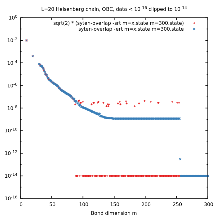
Short answer: Use syten::STensorImpl::STensor::copy() if a copy is unavoidable, move otherwise.
Long answer: Unfortunately, it is rarely quite clear whether an object is copied or moved-from. In particular, constructing a vector from a std::initializer_list of pure r-values, e.g.
produces an unnecessary copy of syten::STensor objects because the content of std::initializer_list is constant, while doing the same with a tuple only produces one move. For a simpler example, see e.g. here, notice how f() constains references to X(X&&) whereas g() contains references to X(X const&).
Furthermore, while returning temporaries inside curly braces into a std::tuple (as e.g. done in syten::STensorImpl::svd) works and does not copy, having named objects there also creates an unnecessary copy, which is not at all reasonable nor quite straightforward to see, as returning a named copy outside a tuple invokes copy elision.
To avoid those and other errors in the future, the copy ctor of syten::STensor logs all implicit copies made using either it or the copy assignment operator if tensor timings are enabled. The public member function syten::STensorImpl::STensor::copy() does not log this and should be used if you are certain that some copy is unavoidable.
The following error is printed when attempting to read a state or lattice file:
terminate called after throwing an instance of 'boost::archive::archive_exception'
  what():  array size too short
This is most likely due to a mismatch between the scalar types used by the toolkit binary (run syten-binary --version to get a printout of its scalar types used) and the file read in. For example, if a lattice is created by syten-sql-mps-spin using real scalar values and then subsequently attempted to be read by syten-random using complex scalar values (or vice versa), the error will occur. See SYTEN_COMPLEX_SCALAR for details.
When reading an input file (e.g. a state or lattice) fails, the following error may be printed:
terminate called after throwing an instance of 'boost::archive::archive_exception'
  what():  input stream error
  Aborted
In this case, you should make sure that you read in a valid state or lattice file. A common reason for failure until recently was to read a file which is still written-to. This failure mode should now be avoided (we create a temporary file first, serialise into that file and then move the temporary file into place), but similar reasons (no space left on device, for example) may also lead to such an error.
The following error is printed when attempting to run a binary (file name may be different):
error while loading shared libraries: libmkl_intel_lp64.so:
  cannot open shared object file: No such file or directory
This error occurs if the system does not find a shared library required by the program. Most likely this will be Boost or the Intel MKL. Make sure that paths to both are contained in your LD_LIBRARY_PATH. At most clusters, the Intel MKL can be enabled by module load intel or module load icc (the version needs to match the version you used to compile the binary). The Boost library can often similarly be loaded via module load or, alternatively, by directly adding the boost/lib directory to your LD_LIBRARY_PATH.
The toolkit stores quantum numbers as syten::HalfInteger values which internally are stored as standard integers of twice the represented value (so a quantum number of Sz=3/2 is stored as an syten::HalfInteger with value 3/2 which in turn is stored as an integer with value 7). By default, a std::int16_t is used as the internal integer storage, resulting in representable quantum numbers ranging from approx. -16'000 to approx. +16'000. For most applications, this is enough.
However, if your lattice is very large and/or bosonic, this may not be enough. Note that in certain applications, such as generation of ‘complete’ random states, enumeration of all possible quantum numbers is necessary.
To alleviate this issue, either choose a smaller lattice or define the macro SYTEN_RDEF_BASE_TYPE to std::int32_t or std::int64_t. Note that the typical concerns apply here, binaries will not be compatible between different values of that type. To do so, add a line CPPFLAGS_EXTRA+=-DSYTEN_RDEF_BASE_TYPE=std::int32_t to your make.inc file.
To pass a complex number as an argument on the command line, use ' around it to stop the shell from intepreting the brackets. Do not place any spaces inside the brackets, i.e., use -d '(0,0.01)', not -d '(0, 0.01)'.
DMRG convergence is currently measured as the relative change of energy over the last two sweeps, something like \(
(E_{\mathrm{last}} - E_{\mathrm{now}})/(|E_{\mathrm{last}}|) \) has to be small. If the energy is exactly zero (or small), this check breaks down. To limit the number of sweeps then, use e.g. (m 50 l 10) for m=50 states and at most l=10 half-sweeps.
This problem can in particular occur if you try to orthogonalise against many orthogonal states or in a small subspace, the eigensolver is then more likely to return a zero state.
syten-random -g s first creates a near-vacuum state (N=0, S=0 etc.) and then applies single-site operators randomly until the state transforms as desired. However, if you attempt to create a S=0 state on five Heisenberg spins (or with e.g. five electrons in the Hubbard model), syten-random -g s will not notice that this is in fact impossible and just try to apply spin flip operators forever. If syten-random -g s takes suspiciously long, consider re-checking your arguments. Alternatively, the ‘complete’ generator -g c will generate a zero-norm state in this case (all tensors empty).
If your program needs more memory than the operating system can supply, it may either throw a std::bad_alloc exception (if the OS denies an allocation) or get killed by a SIGKILL signal (if the OS initially agreed to the allocation but doesn’t have the memory once we access it, cf. overcommit.)
To diagnose such problems, you should
SYTEN_TENSOR_TIME=t and SYTEN_LOG_TIME_LVL=6. The former will cause timing of all tensor products to be enabled, the latter will print out the times after each individual product. In this way, you can check which product in your code is the problematic one, the last ‘completed’ product will be printed out just before the crash. The output tells you the line of the product as well as the sizes (in blocks and memory) of the involved tensors.SYTEN_MEMORY_SAMPLER=mysamplefile. This will cause memory usage to be printed to the file continously. You can cross-check with the output of the tensor timer to see which products and at which times your code needs the most memory.Once you have identified the parts of the code taking the most memory, you should check that only temporary tensors necessary during specific tensor contractions exceed the memory budget of your computer. If (e.g.) individual MPS tensors already go beyond the RAM available, there is not much one can do. If you have identified some temporary tensors which need a lot of RAM, you might want to
syten::correct_cgc_tensors on high-rank tensors periodically to avoid a build-up of errors in the CGC tensors.A*B*C, sometimes A and sometimes C is bigger (and B in each case reduces the size considerably), it may be preferably to sometimes do (A*B)*C (if A is bigger) and sometimes do A*(B*C) (if C is bigger). syten::MemoryUsage::totalSize may help you determine the size of each tensor, alternatively, comparing the sizes of the relevant bonds may be more appropriate.syten::STensor or having equal-rank syten::Tensor objects: If you get warnings like
or
these are due to unexpected situations in the asynchronous caching subsystem. This subsystem receives requests to cache or uncache specific objects and then dispatches workers to do so asynchronously. If a request to uncache an object comes in while this object is still being cached to disk, a performance hit is to be expected (as we have to wait until the caching process completes before we can undo it). You can enable/disable caching using the List of Environment Variables SYTEN_DO_CACHE and friends and you may also adapt the number of workers used and the caching threshold applied (to avoid caching very small objects).
While this warning may be annoying, it normally should not hint towards any kind of calculational error, the most likely cause is that the hard disk drive is much slower than expected.
If you get error messages like
or observe a deadlock in the mutex protecting a CUDA dense tensor product:
and your glibc version is very old (e.g. 2.22 as shipped by OpenSUSE and used on some clusters), try updating the version of glibc used. At least in one case, it was (a) not possible to reproduce the issue with identical settings and compilers except for a newer glibc and (b) updating glibc on the same cluster solved the problem.
When trying to reproduce an issue and failing, make sure that settings which may affect runtime behaviour are checked, in particular:
make.inc file used to compile is identical or that all differences are understoodenv on both systems is identical in particular with respect to LD_LIBRARY_PATH and LD_PRELOAD variableswhich syten-dmrg)--version and, if necessary, --version-diff switches).Linking the pyten module against libtcmalloc causes Python exceptions to produce very long and uncompletely unusable error messages. Try again without linking against libtcmalloc.
Clebsch-Gordan tensors are used to store the relation between multiplets of states with non-abelian symmetry. During a long calculation, it is possible that errors accumulate in those tensors which lead to non-physical results. Such errors are detected by (among others) contracting the tensor with itself over all but one leg, a proper CGC (of any rank) will give a result proportional to the identity matrix. On every SVD, this contraction is required anyways to ensure proper normalisation and it is straightforward to check for validity of the tensor. Furthermore, tensor products should either be of order one or exactly zero – if they are very small, this also indicates a loss of precision.
Under those circumstances, you will get warning messages likes
or
The first message indicates that a small CGC tensor was observed, the second message that a non-physical CGC tensor was found (here combining a one-dimensional singlet and a two-dimensional doublet into a four-dimensional quadruplet, which is impossible).
In connection with those error messages, you may also observe your program to get stuck without visible progress and/or extremely high memory usage. This is due to those imprecise CGC spaces no longer being parallel to each other and hence not allowing the reduction of parallel tensor blocks in a tensor. As a result, the number of blocks in each tensor and the memory usage explode.
The high-precision scalars used by SyTen mean that in most cases, you will never run into these problems. However, if your calculations are particularly long and/or your tensor rank is relatively high and/or you are working with large-spin states, you might exhaust the precision of those scalars eventually. Fortunately, it is possible to stabilise even long-running calculations by periodically re-constructing the CGC tensors from scratch. This is done by merging all incoming and outgoing legs into one large leg, ensuring that the resulting rank-2 tensor is proportional to the identity and de-merging the legs again (using exact rank-3 fusing/splitting tensors). The function syten::correct_cgc_tensors() takes care of this and you may wish to call it from time to time, ideally on relatively small tensors carrying the calculation forward. For example, you might want to call it on the tensors of a MPS during a long time evolution, but there is (typically) no reason to call it on the intermediate tensor of e.g. a local eigensolver problem.
For examples of this being done, see e.g. inc/mps/tdvp.cpp or the iPEPSv1 code.
Note that while the C++ function syten::correct_cgc_tensors() takes its argument by reference and works on it in-place, the Python function returns the corrected CGC tensor, taking its argument by-value.
In OpenMP 5.0, the function omp_set_nested() to enable nested parallelisation is deprecated. In OpenMP 4.5, it is necessary to call it to enable nested parallelisation. Unfortunately, while both GCC and Clang at the moment do not implement OpenMP 5.0 and hence define the _OPENMP macro to be smaller than 201611 (for OpenMP 5.0 Preview 1), the libiomp5 library shipped with Clang 9.0 already implements this preview and prints a warning if we use omp_set_nested().
This means that while we check the value of the _OPENMP macro at compile-time to only call omp_set_nested() if the OpenMP version is 4.5 or earlier, this does not suffice to ensure that the same version is used at runtime. Unfortunately, OpenMP does not define an interface to get the version of the linked runtime at runtime.
With GCC 8.2, it is recommended to link in libiomp5, as libgomp has performance issues; then using a recent libiomp5 will print the warning. With Clang 9.0, the same problem exists when using the shipped libiomp5. GCC 9.x throws up when used together with libiomp5, hence for this version of GCC, one should only link in libgomp and the problem will not occur.
In any case, this is only a warning which may be annoying but does not hurt. It will go away as soon as the compilers implement OpenMP 5.0 and hence set the _OPENMP macro correctly.
For GCC 8.x and earlier, it is recommended to link in both the Intel-provided libiomp5 and the GNU-provided libgomp as OpenMP runtime libraries, with libiomp5 linked in first and taking precedence. This is because libgomp suffers from some severe performance problems and does not appear to keep a thread pool. However, starting with GCC 9.x, the compiler produces erroneous code when linked with libiomp5, you should hence not link in libiomp5 when using GCC 9.x. Furthermore, when using then Intel MKL together with GCC 9.x, make sure to use -lmkl_gnu_thread and not -lmkl_intel_thread (cf. make.inc.example).
OpenBLAS in version 0.2.20 defines its complex functions to take float and double pointers whereas all other BLAS libraries take void pointers (cf. here). This was fixed in a later release.
The problem is likely to surface while compiling e.g. inc/util/dynarray.cpp.
If possible, please install a later release of OpenBLAS. If you are stuck on a buggy OpenBLAS installation, please
/etc/alternatives/cblas.h-x86_64-linux-gnu to point to /usr/include/x86_64-linux-gnu/cblas-netlib.h)SYTEN_USE_OPENBLAS macro (the generic header does not have the OpenBLAS-specific threading functions).The compiler emits an error message complaining e.g. about
if constexpr (is_number<decltype(r)>::value) {
   ^~~~~~~~~
Starting at commit f366cfad, SyTen requires a C++17 compatible compiler, such as GCC 7.x. If your compiler is older and you cannot upgrade, consider the last C++11-commit only, tagged as pre-C++17: git checkout pre-C++17.
GCC 7.1 incorrectly diagnoses a strict-aliasing violation (GCC 7.2 fixes this problem). To avoid the error message, add CPPFLAGS_EXTRA+=-Wno-strict-aliasing to your make.inc file.
If you encounter such an error, it is most likely because you still have an old dependency file which refers to a no-longer existing header file. Make then tries to re-make this header file, but does not know how (since they are written by hand, not by make) and then stops. Try to delete all old header files, e.g. via
find . -name '*.d' -delete
executed in the toolkit directory.
This error occurs if you compiled object files with the Intel compiler, but then attempted to compile an executable using either GCC or Clang. Either use the Intel compiler to also compile the executable or re-compile the object files with the other compiler. This can be done easiest by deleting all old object files via
find . -name '*.o' -delete
GCC 6.x does not yet know about the [[fallthrough]] attribute which is a part of C++17. If you encounter this error, it is best to silence the warning by adding the line
CPPFLAGS_EXTRA+=-Wno-attributes
to your make.inc file.
The following error is emitted by the linker:
/usr/lib/../lib64/crt1.o: In function `_start':
  /usr/src/packages/BUILD/glibc-2.11.3/csu/../sysdeps/x86_64/elf/start.S:109:
  undefined reference to `main'
This complains that there is no function main() when attempting to build an executable. Most likely the error occurs because you only declared a function syten::main(). To be precise, an executable should follow either this model:
or
The first method is slightly preferred because it minimises the use of the global namespace and hence possibly name clashes with other functions.
Please see Contributors.